Scanner models
A scanner is one constructor call: EICTScanner(; …) for an energy-integrating scintillator detector or PCCTScanner(; …) for a photon-counting direct-conversion detector. Both compose the same ScannerGeometry, whose fields read straight off the scanner (scanner.source_to_isocenter), and each rejects the other family's keywords.
Overview
There are no preset factory functions in the package. The clinical systems below are the documented parameter sets that the example notebooks pass to the constructors, reproduced keyword for keyword, so any of them can be pasted into a session. Parameters a vendor does not publish are marked as modelling assumptions, as the notebooks mark them.
| System | Constructor | Detector | Notebooks |
|---|---|---|---|
| GE Revolution Apex Elite | EICTScanner | Gemstone garnet, MC LUT (:lumex) | 01, 02, 03, 05, 06, 07 |
| Siemens NAEOTOM Alpha | PCCTScanner | CdTe 1.6 mm, 4 thresholds | 04, 08 |
| Siemens SOMATOM Force | EICTScanner | UFC Gd₂O₂S, MC LUT (:ufc) | 09 |
| Siemens SOMATOM Definition Flash | EICTScanner | UFC Gd₂O₂S, Flash MC LUT (:ufc_flash) | 12 |
| Research geometries | EICTScanner | Gemstone (:lumex) | 10, 11 |
Anything that changes between scans (kVp, mA, views, rotation time, collimation, pitch, added filters such as a tin shield) belongs in CTProtocol, not in the scanner. A dual-source system is modelled as two acquisitions: one scanner per tube/detector chain, each with its own protocol.
Constructor defaults
Every keyword has a default (a CatSim-like research scanner), so EICTScanner() alone is valid; PCCTScanner additionally requires energy_thresholds. Distances are in mm, detector sizes are at the isocentre.
Geometry — both families
| Keyword | Default | Meaning |
|---|---|---|
| source_to_isocenter | 540.0 | source-to-isocentre distance (SID), mm |
| source_to_detector | 950.0 | source-to-detector distance (SDD), mm |
| detector_rows × detector_cols | 64 × 900 | physical detector array |
| detector_row_size / detector_col_size | 1.0 / 1.0 | element size at isocentre, mm |
| detector_row_offset | 0.0 | row offset, rows |
| detector_col_offset | 0.25 | quarter-detector offset, columns (rays of opposing views interleave) |
| detector_shape | :arc | :arc (equiangular, focal-spot-centred) or :flat |
| focal_spot_width / focal_spot_length | 1.0 / 1.0 | focal spot, mm |
| target_angle | 7.0 | anode angle, degrees |
| gantry_rotation_time | 0.5 | s |
| scan_diameter / gantry_aperture | 500.0 / 700.0 | scan field and bore, mm |
| flat_filter_material / flat_filter_thickness | :aluminum / 2.0 | built-in flat filter, mm |
| bowtie_filter | :large_body | see the bowtie catalog below |
EICTScanner — scintillator
| Keyword | Default | Meaning |
|---|---|---|
| detector_material | :lumex | selects the detector-efficiency model |
| detector_depth | 3.0 | scintillator depth, mm (used by the Beer–Lambert fallback only) |
| fill_factor_row / fill_factor_col | 0.9 / 0.9 | active-area fraction |
| detection_gain | 15.0 | electrons per keV |
| electronic_noise | 5000.0 | DAS noise σ, electrons, added to the counts before the log |
PCCTScanner — direct conversion
| Keyword | Default | Meaning |
|---|---|---|
| energy_thresholds | required | keV, ascending; one counting bin per threshold |
| n_energy_bins | length(energy_thresholds) | must equal the threshold count |
| detector_material / detector_depth | :CdTe / 1.6 | :CdTe, :CZT or :Si; mm |
| fill_factor_row / fill_factor_col | 0.9 / 0.9 | active-area fraction |
| energy_resolution | 0.0 | FWHM, keV |
| charge_sharing_fwhm | 0.0 | charge-cloud FWHM, mm |
| dead_time_ns | 0.0 | pulse dead time; pile-up is modelled only when > 0 |
| pixel_mode | :standard | :standard, :uhr or :macro |
| native_dexel_col_mm / native_dexel_row_mm | 0 / 0 | native dexel at the detector face; 0 infers it from the binned pixel |
| binning_factor | 1 | spatial binning of native dexels |
| pileup | true | Monte Carlo pile-up (needs dead_time_ns > 0) |
| pileup_correction | false | model-based inverse of the pile-up on the recorded bins |
| scatter_correction | false | model-based scatter estimate-and-subtract on the bins |
| noise_reduction | 0.0 | count-noise blend, 0 = Poisson counts … 1 = expected counts |
Detectors, bowties, filters
Energy-integrating detector materials
With SimOptions(use_detector_efficiency = true) (the default) the energy-integrating forward model weights every energy by a Monte Carlo absorbed-fraction table η(E), 1–140 keV. detector_efficiency_mode = :beer_lambert switches to the analytical fallback, which is the only place detector_depth matters. Any other material symbol is an error.
| detector_material | Scintillator | η(E) table | Fallback depth |
|---|---|---|---|
| :lumex | GE Gemstone Ce:(Tb,Lu)₃Al₅O₁₂ garnet | GEMSTONE_MC_EFFICIENCY_LUT | 3.0 mm |
| :ufc | Siemens UFC Gd₂O₂S:Pr,Ce (SOMATOM Force) | UFC_MC_EFFICIENCY_LUT | 1.4 mm |
| :ufc_flash | Siemens UFC Gd₂O₂S:Pr,Ce (SOMATOM Definition Flash) | UFC_FLASH_MC_EFFICIENCY_LUT | 1.0 mm |
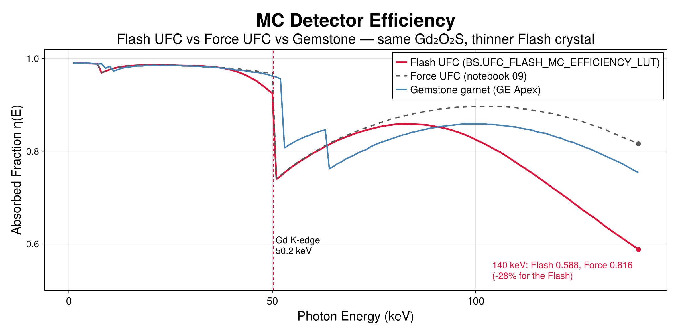
The garnet table carries the Tb (52.0 keV) and Lu (63.3 keV) K-fluorescence escape dips; the two UFC tables carry the Gd K-edge escape at 50.2 keV. The Flash crystal is thinner than the Force's: the two tables agree below 30 keV and differ by −28 % at 140 keV (0.588 vs 0.816), and a test forbids aliasing them.
Photon-counting sensors
:CdTe, :CZT and :Si. The photon-counting chain always applies a Monte Carlo detector-response matrix (photoelectric, Compton and Rayleigh transport, Fano noise, charge sharing, K-fluorescence) before thresholding into bins, then the Monte Carlo pile-up and the optional pile-up and scatter corrections set on the scanner.
Bowtie filters
| bowtie_filter | Profile |
|---|---|
| :large_body (:ge_revolution_large) | CatSim/XCIST large-body profile |
| :medium_body (:ge_revolution_medium) | CatSim/XCIST medium-body profile |
| :small_body (:ge_revolution_small) | CatSim/XCIST small-body profile |
| :head | generic head profile |
| :none | no bowtie |
Filtration
The scanner's flat filter is flat_filter_material (:aluminum, :copper or :titanium) at flat_filter_thickness mm. Per-scan layers go on the protocol: CTProtocol(additional_filters = [("Ti", 0.9), ("Sn", 0.6)]) accepts "Al", "Cu", "Sn", "Ti", "C" and "W". Source spectra are the bundled IPEM tables at 8° and 10° anode angles (CTProtocol(anode_angle = 8)), up to 140 kVp.
GE Revolution Apex Elite
A 256-row wide-cone system with 0.625 mm rows and a curved Gemstone (Lumex) garnet array. Notebooks 01, 02 and 05 add clinical DAS noise (3500 e⁻); the VMI and CatSim notebooks (03, 06, 07) set electronic_noise = 0.
scanner = BS.EICTScanner(
    source_to_isocenter = 625.6,  source_to_detector = 1100.0,
    detector_rows = 256,          detector_cols = 834,
    detector_row_size = 0.625,    detector_col_size = 0.6,
    detector_col_offset = 0.25,   detector_shape = :arc,     # the defaults, written out
    focal_spot_width = 1.0,       focal_spot_length = 1.0,   target_angle = 10.0,
    flat_filter_material = :aluminum, flat_filter_thickness = 2.5,
    bowtie_filter = :ge_revolution_large,
    detector_material = :lumex,   detector_depth = 3.0,
    fill_factor_row = 0.9,        fill_factor_col = 0.9,
    electronic_noise = 3500.0,    # e⁻, clinical DAS readout (0 in the VMI notebooks)
    detection_gain = 10.0,        # e⁻/keV
)| Protocol (as run) | kVp | mA | Views / rotation | Collimation | Added filter |
|---|---|---|---|---|---|
| Single energy (01, 05) | 120 | 200 / 250 | 500 / 1.0 s | 5 mm | Al 4.5 mm |
| Rapid kVp switching (03, 07) | 80 / 140 | (407 × 0.65 / 405 × 0.35) × DOSE_SCALE | 984 / 0.5 s | 5 mm | Al 4.5 mm |
Rapid kVp switching is each energy's duty cycle of the view: 0.65 of the view period at 80 kVp and 0.35 at 140 kVp, for the tube current and for the arc the view integrates over (view_arc). DOSE_SCALE scales both to the physical scan's CTDIvol of 10.07 mGy. Every notebook integrates each view over its arc with SimOptions(; view_samples = 5) (CatSim's comparison in 06 uses point views on both sides).
Siemens NAEOTOM Alpha
The photon-counting system. Native CdTe dexels of 0.275 × 0.322 mm at the detector face are binned 2 × 2, which at the 1113/610 magnification gives 0.301 × 0.353 mm pixels at the isocentre and 144 rows; notebooks 04 and 08 both span the 50 cm scan field (1659 columns). Four thresholds at 20, 35, 55 and 70 keV make the bins 20–35, 35–55, 55–70 and > 70 keV.
scanner = let native_col = 0.275, native_row = 0.322,   # mm at the detector face
               sid = 610.0, sdd = 1113.0, bf = 2
    col_iso = native_col * bf / (sdd / sid)                # 0.301 mm
    row_iso = native_row * bf / (sdd / sid)                # 0.353 mm
    BS.PCCTScanner(
        source_to_isocenter = sid, source_to_detector = sdd,
        detector_rows = 144, detector_cols = ceil(Int, 500.0 / col_iso),   # the 50 cm scan field
        detector_row_size = row_iso, detector_col_size = col_iso,
        detector_shape = :arc, detector_col_offset = 0.25,
        focal_spot_width = 0.4, focal_spot_length = 0.5, target_angle = 7.0,
        gantry_rotation_time = 0.5, scan_diameter = 500.0, gantry_aperture = 820.0,
        flat_filter_material = :aluminum, flat_filter_thickness = 3.0,
        bowtie_filter = :large_body,                        # both notebooks
        detector_material = :cdte, detector_depth = 1.6,
        fill_factor_row = 0.95, fill_factor_col = 0.95,
        energy_thresholds = [20.0, 35.0, 55.0, 70.0],
        energy_resolution = 10.0, charge_sharing_fwhm = 0.08, dead_time_ns = 5.0,
        pixel_mode = :standard,
        native_dexel_col_mm = native_col, native_dexel_row_mm = native_row, binning_factor = bf,
        pileup_correction = true, scatter_correction = true, noise_reduction = 0.0,
    )
end
Both notebooks scan at 140 kVp and 174 mA × DOSE_SCALE (the physical CTDIvol of 10.12 mGy), 1200 views in 0.5 s, 5 mm collimation, with the tube's 0.9 mm titanium window as additional_filters = [("Ti", 0.9)] on top of the 3 mm aluminium, exact Poisson counts, and view integration on the photon-counting path (view_samples = 5).
Siemens SOMATOM Force
Third-generation dual source: 96 rows of 0.6 mm (57.6 mm), 920 channels of 0.054° (0.561 mm at the isocentre). Both tubes use tube A's geometry so the low/high sinogram pair is co-registered ray by ray; the Gammex body fits inside detector B's real 35.5 cm field, so no ray used would be missing on the real detector.
scanner = BS.EICTScanner(
    source_to_isocenter = 595.0, source_to_detector = 1085.6,
    detector_rows = 96,          detector_cols = 920,
    detector_row_size = 0.6,     detector_col_size = 0.561,
    focal_spot_width = 0.8,      focal_spot_length = 1.2,  target_angle = 8.0,
    flat_filter_material = :aluminum, flat_filter_thickness = 3.0,
    bowtie_filter = :large_body,                 # assumption: Siemens profile unpublished
    detector_material = :ufc,    detector_depth = 1.4,
    fill_factor_row = 0.9,       fill_factor_col = 0.9,
    electronic_noise = 0,        detection_gain = 10.0,
)
protocol_low  = BS.CTProtocol(kVp = 100, mA = 380.0, views = 1160, rotation_time = 0.5,
                              collimation_mm = 4.8, anode_angle = 8,
                              additional_filters = [("Ti", 0.9)])
protocol_high = BS.CTProtocol(kVp = 140, mA = 190.0, views = 1160, rotation_time = 0.5,
                              collimation_mm = 4.8, anode_angle = 8,
                              additional_filters = [("Ti", 0.9), ("Sn", 0.6)])
The clinical abdomen pairs are x/Sn150; the bundled spectra stop at 140 kVp, so the notebook runs 100/Sn140 at the published 2:1 current ratio. Assumptions: 8° anode, 3.0 mm Al + 0.9 mm Ti flat filtration (the Vectron-family stack), the CatSim large-body bowtie, 1.4 mm crystal and zero electronic noise. The 0.88 mm tube-B z-offset is applied by shifting the phantom.
Siemens SOMATOM Definition Flash
Second-generation dual source (2008). Two STRATON MX P tubes and two UFC detectors, 95° apart. The detector efficiency is its own Monte Carlo table, UFC_FLASH_MC_EFFICIENCY_LUT (detector_material = :ufc_flash), not the Force's: same Gd₂O₂S material, thinner crystal. The sourced specification follows; unpublished items are listed as assumptions.
Identification
| Item | Value |
|---|---|
| FDA 510(k) | K082220 (10/2008, SOMATOM Flash DS); Stellar detector variant K113342 (12/2011); VA44 + 0.5 mm slices K121072 (2012); later K122471, K173630, K230421 |
| Product code / class | 90 JAK, Class II, 21 CFR §892.1750 |
Gantry geometry
| Parameter | Value | Source |
|---|---|---|
| SID / SDD | 595.0 / 1085.6 mm (magnification 1.8245) | DICOM-CT-PD / AAPM LDCT projection data |
| Detector shape | arc, equiangular, focal-spot-centred | LDCT-PD |
| Tube A ↔ tube B offset | 95° (94° also appears in the literature) | technical reviews |
| Bore / scan field (A) | 78 cm / 50 cm (78 cm extended FOV option) | Siemens datasheet 2010 |
| Gantry tilt | none | NHS attribute sheet |
Detector
| Parameter | Detector A | Detector B |
|---|---|---|
| Elements (datasheet: 77,824 total) | 47,104 | 30,720 |
| Rows × channels | 64 × 736 | 64 × 480 |
| Column pitch at detector / isocentre | 1.2858 / 0.70473 mm | same |
| Fan angle / FOV at isocentre | 49.94° / 50.2 cm | 32.57° / 33.4 cm |
| Row pitch at isocentre / z-coverage | 0.6 mm / 38.4 mm | same |
| Slices per rotation | 2 × 128 with z-Sharp flying focal spot | |
| Scintillator | UFC Gd₂O₂S:Pr,Ce (ρ ≈ 7.34 g/cm³); Stellar (2011+) integrates the ASIC in the photodiode |
Tubes and filtration
| Parameter | Value |
|---|---|
| Tubes / generator | 2 × STRATON MX P, 2 × 100 kW |
| kV steps | 80, 100, 120, 140 (70 on later software) |
| Tube current | 20–800 mA single source; 40–1600 mA dual source |
| Focal spots (IEC 60336) | 0.7 × 0.7 mm and 0.9 × 1.1 mm, 7° anode |
| Flat filtration | 6.8 mm Al eq. (tube) + 1.6 mm Al eq. (beam-limiting device) = 8.4 mm Al eq.; +0.5 mm Al mode-dependent CARE Filter |
| Selective Photon Shield | 0.4 mm Sn on the high-kV tube (Primak et al., AJR 2010) |
| Bowtie | shaped form filters, profile unpublished |
| Dual-energy pairs | 80/Sn140 and 100/Sn140 kV; liver VNC 100/Sn140 at 230/178 quality-reference mAs, 32 × 0.6 mm |
Acquisition
| Parameter | Value |
|---|---|
| Rotation | 0.28 (optional), 0.33, 0.5, 1.0 s |
| Temporal resolution | 75 ms, heart-rate independent |
| Projections | up to 4,608 per 360° per acquisition unit; 1,152 per focal-spot position at 0.5 s (2,304 with z-FFS) |
| Pitch | 0.35–3.0 routine; up to 3.2 (3.4 ECG-triggered) Flash Spiral |
| Collimations | 2 × 128 × 0.6 mm dual source; 128/64/40/32/20/16/10/8 × 0.6 and 32 × 1.2 mm single source |
| Vendor reconstruction | SAFIRE, later ADMIRE; iMAR; 512² matrix |
The model
scanner = BS.EICTScanner(                     # tube/detector A, used for both tubes
    source_to_isocenter = 595.0, source_to_detector = 1085.6,
    detector_rows = 64,          detector_cols = 736,
    detector_row_size = 0.6,     detector_col_size = 0.70473,
    detector_shape = :arc,
    focal_spot_width = 0.7,      focal_spot_length = 0.7,  target_angle = 7.0,
    gantry_rotation_time = 0.5,  scan_diameter = 500.0,    gantry_aperture = 780.0,
    flat_filter_material = :aluminum, flat_filter_thickness = 8.4,
    bowtie_filter = :large_body,                 # assumption: profile unpublished
    detector_material = :ufc_flash,              # the Flash table, never :ufc
    detector_depth = 1.0,
    fill_factor_row = 0.9,       fill_factor_col = 0.9,
    electronic_noise = 1500,     # e⁻, Stellar DAS floor (pre-2011 builds ≈ 3500)
    detection_gain = 10.0,
)
# dual energy: 80 kV on tube A, Sn140 on tube B; a full 1152-view rotation each, both currents
# scaled by DOSE_SCALE to the physical scan's CTDIvol (10.01 mGy)
protocol_low  = BS.CTProtocol(kVp = 80, mA = 470.0 * DOSE_SCALE, views = 1152, rotation_time = 0.5,
                              collimation_mm = 4.8, anode_angle = 8)
protocol_high = BS.CTProtocol(kVp = 140, mA = 182.0 * DOSE_SCALE, views = 1152, rotation_time = 0.5,
                              collimation_mm = 4.8, anode_angle = 8,
                              additional_filters = [("Sn", 0.4)])
The heel effect is off and every view integrates over its arc (view_samples = 5). Notebook 12 also runs the regular dual-power mode, 120 kV on both tubes at 420 mA × DOSE_SCALE each, whose two independent chains reduce noise by √2. The bundled spectra reach 140 kVp, the Flash's top kV, so the clinical pair runs without substitution; they come at 8° and 10° anodes, so the published 7° is run as 8°.
Modelling assumptions
| Item | Status | Choice |
|---|---|---|
| Bowtie profile | unpublished | CatSim :large_body |
| Flat-filter composition | only the Al equivalent is published | 8.4 mm Al equivalent |
| UFC layer depth | proprietary | 1.0 mm (inert with the MC table) |
| Fill factor | proprietary | 0.9 (cancels in the air calibration) |
| Electronic noise | never published | 1500 e⁻ Stellar; ≈ 3500 e⁻ pre-2011 |
| Tube-B z-offset | not published for the Flash | 0 (no-op for z-invariant phantoms) |
| Detector B truncation | real: 33 cm | tube B uses the A arc for a ≤ 33 cm phantom, so the pair is co-registered |
Research geometries
Two notebooks use generic geometries and leave the rest at the defaults: the titanium-implant study (a compact 16-row scanner) and the helical study (a 256 × 0.625 mm, 16 cm wide-cone volume scanner, scanned with 20 mm collimation at pitch 1.0).
scanner_implant = BS.EICTScanner(            # notebook 10
    source_to_isocenter = 540.0, source_to_detector = 950.0,
    detector_rows = 16, detector_cols = 512,
    detector_row_size = 1.0, detector_col_size = 1.0,
    detector_material = :lumex, detector_depth = 3.0,
)
scanner_helical = BS.EICTScanner(            # notebook 11
    source_to_isocenter = 541.0, source_to_detector = 949.0,
    detector_rows = 256, detector_cols = 512,
    detector_row_size = 0.625, detector_col_size = 1.0,
)
helical = BS.CTProtocol(kVp = 120.0, mA = 200.0, views = 360, rotation_time = 0.5,
                        collimation_mm = 20.0, pitch = 1.0, n_rotations = 16)
Modelling a new scanner
What a new system needs, in three tiers.
| Tier | Where | What |
|---|---|---|
| A — required | EICTScanner / PCCTScanner | SID and SDD; physical rows × columns and element size at the isocentre (column size at iso = pitch at the detector ÷ magnification); detector shape; focal spot and anode angle; rotation time, scan field, bore; flat filter and bowtie; the detector material, which must map to an existing η(E) table (or a new Monte Carlo run); fill factors; for photon counting, the thresholds, resolution, charge sharing, dead time, native dexel and binning. |
| B — protocol | CTProtocol | kVp list; mA range; rotation time; views per rotation; collimation options; mode-dependent added filters (e.g. tin); pitch range. |
| C — unpublished | documented assumptions | bowtie profile, scintillator depth, fill factor, absolute electronic noise, exact filter stack, tube-B z-offset. State each one in the notebook, as notebooks 09 and 12 do. |
Check a protocol against the hardware with validate_protocol(protocol, scanner), and the detector rows an axial reconstruction needs with required_axial_detector_rows(scanner; fov_cm, z_cm).